Zimmer

Description

Zimmer’s Effective Dose Model (EDM) is a parametric synergy model. This model uses the multiplicative survival principle (i.e., Bliss), but adds a parameter for each drug describing how it affects the potency of the other. Specifically, given doses \(d_1\) and \(d_2\), this model translates them to “effective” doses using the following system of equations

\[d_{1, \text{eff}} := \frac{d_1}{1 + a_{12}\left(\frac{1}{1 + \left(\frac{d_{2, \text{eff}}}{C_2}\right)^{-1}}\right)}\]

\[d_{2, \text{eff}} := \frac{d_2}{1 + a_{21}\left(\frac{1}{1 + \left(\frac{d_{1, \text{eff}}}{C_1}\right)^{-1}}\right)}\]

In addition to those equations, the EDM assumes each single drug follows a 2-parameter Hill equation synergy.single.hill.Hill2P(E0=1, Emax=0).

The values of Effective Dose Model synergy parameters are interpreted as

Parameter	Values	Synergy/Antagonism	Interpretation
\(a_{12}\)	\((-\frac{C_2}{d_{2,\text{eff}}} - 1, 0)\)	Synergism	Drug 2 increases the effective dose (potency) of drug 1
	\(> 0\)	Antagonism	Drug 2 decreases the effective dose (potency) of drug 1
\(a_{21}\)	\((-\frac{C_1}{d_{1,\text{eff}}} - 1, 0)\)	Synergism	Drug 1 increases the effective dose (potency) of drug 2
	\(> 0\)	Antagonism	Drug 1 decreases the effective dose (potency) of drug 2

Assumptions

Each individual drug follows a Hill equation dose response with E0=1 and Emax=0
All effect values fall within [0, 1]

If these assumptions are not met, you may consider using another synergy model based on the multiplicative survival principale, such as Bliss or ZIP, or another model including some form of synergistic potency, such as MuSyC or BRAID.

Defaults

Single-drug models
- Default: synergy.single.hill.Hill2P(E0=1, Emax=0)
- Required: synergy.single.hill.Hill2P or subclass

Load and plot example dataset

2D synergy models work with 1D arrays of drug 1 dose, drug 2 dose, and effect.

[1]:

from synergy import datasets
from synergy.utils.plots import plot_heatmap, plot_surface_plotly, set_plotly_interactive

set_plotly_interactive()  # This should only be run in an interactive notebook setting - for other scripts skip this

d1, d2, E = datasets.load_2d_example()

Fit the Zimmer model to data

[2]:

from synergy.combination.zimmer import Zimmer

model = Zimmer()
model.fit(d1, d2, E, bootstrap_iterations=100, use_jacobian=False)  # bootstrap iterations is used to get confidence intervals
model.summarize()

Parameter  |  Value   |  95% CI           |  Comparison  |  Synergy
=======================================================================
a12        |  -0.872  |  (-1.05, -0.277)  |  < 1         |  synergistic
a21        |  -0.876  |  (-1.25, -0.327)  |  < 1         |  synergistic

[3]:

for parameter, ci in model.get_confidence_intervals().items():
    print(f"{parameter}: {ci}")

h1: [0.43866078 0.59074892]
h2: [0.51304362 0.65726413]
C1: [ 7.24345507 12.13209283]
C2: [2.0312226  2.95592122]
a12: [-1.05202436 -0.2771949 ]
a21: [-1.24706193 -0.32749117]

Plot the model fit

[4]:

from synergy.utils.dose_utils import make_dose_grid

# Get a smooth looking dose response surface from dmin=0.025 to dmax=20
dmin, dmax = 0.025, 20
n_points = 20  # 20 points x 20 points
d1_smooth, d2_smooth = make_dose_grid(dmin, dmax, dmin, dmax, n_points, n_points)
E_smooth = model.E(d1_smooth, d2_smooth)

scatter_points = {
    "drug1.conc": d1,
    "drug2.conc": d2,
    "effect": E
}

plot_surface_plotly(d1_smooth, d2_smooth, E_smooth, cmap="YlGnBu", title="Zimmer Fit", scatter_points=scatter_points)

[5]:

from matplotlib import pyplot as plt
import numpy as np

from synergy.utils.dose_utils import aggregate_replicates

# plot_heatmap will automatically aggregate replicates for real data, but we don't need it to do that for the BRAID fit (middle plot)
d, _ = aggregate_replicates(np.vstack([d1, d2]).transpose(), E)
unique_d1 = d[:, 0]
unique_d2 = d[:, 1]

fig = plt.figure(figsize=(10, 5))
plot_heatmap(d1, d2, E, title="Original Data", cmap="YlGnBu", ax=fig.add_subplot(1, 3, 1))
plot_heatmap(unique_d1, unique_d2, model.E(unique_d1, unique_d2), title="Zimmer Fit", cmap="YlGnBu", ax=fig.add_subplot(1, 3, 2))
plot_heatmap(d1, d2, model.E(d1, d2) - E, title="Residuals", cmap="RdBu", ax=fig.add_subplot(1, 3, 3), center_on_zero=True)
plt.tight_layout()

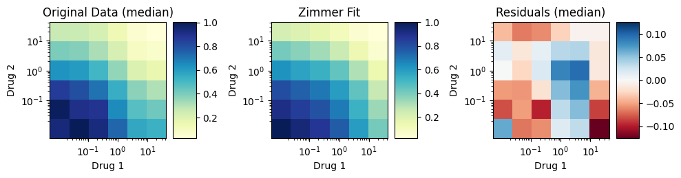
../../_images/models_synergy_zimmer_8_0.png

Notice the Zimmer residuals do not appear random. This is because the synthetic dataset synergy.datasets.load_2d_example() was generated using drugs with \(E_0 = 1\), but NOT \(E_{max} = 0\) as is assumed by the Zimmer equations. The model fit erroneously accounts for this by underestimating the drugs’ Hill coefficients \(h_i\). When data like this are encountered, alternative synergy models based on the multiplicative survival principal may be considered. For instance MuSyC is a related model which also computes synergistic potency. Conversely, models such as Bliss or ZIP may be used to find dose-dependent synergy.

N-drug Combinations

The EDM has not been generalized to an \(N\)-drug case

References

Zimmer, A., Katzir, I., Dekel, E., Mayo, A. E., & Alon, U. (2016). Prediction of multidimensional drug dose responses based on measurements of drug pairs. Proceedings of the National Academy of Sciences of the United States of America, 113(37), 10442–10447. https://doi.org/10.1073/pnas.1606301113

[ ]: