BRAID

Description

BRAID is a parametric synergy model based on the Loewe additivity principle. In BRAID, synergy is parametrically defined using the parameters kappa and delta, another parameter, E3 is also related to the overall strength of the combination.

Note: E3 is not defined as \(\lim_{d_1 \rightarrow \inf, d_2 \rightarrow \inf}E(d_1, d_2)\) in BRAID.

BRAID models multidimensional drug response data using a form based on the Hill equation

\[E_{braid}(d_1, d_2) := E_0 + \frac{\Delta_{max} E}{1 + D(d_1, d_2)^{-\delta \cdot h}}\]

where \(\Delta_{max} E\) is based on the undrugged state \(E_0\), the maximum effect of drugs 1 (\(E_1\)) and 2 (\(E_2\)), as well as a parameter fit by the model \(E_3\)

\[\Delta_{max} E := \max\left(|E_1 - E_0|, |E_2 - E_0|, |E_3 - E_0|\right)\]

Note \(E_3\) has no impact on the model unless it represents a stronger effect than either \(E_1\) or \(E_2\).

\(h\) is the geometric mean of the individual drugs’ Hill coefficients

\[h := \sqrt{h_1 \cdot h_2}\]

and \(D(d_1, d_2)\) is an “aggregate” dose defined as

\[D(d_1, d_2) := D_1^{\frac{1}{\delta h}} + D_2^{\frac{1}{\delta h}} + \kappa \sqrt{\left(D_1^{\frac{1}{\delta h}}\right)\left(D_2^{\frac{1}{\delta h}}\right)}\]

where

\[D_i(d_i) := \frac{\left(\frac{E_i - E_0}{\Delta_{max} E}\right)\left(\frac{d_i}{C_i}\right)^{h_i}}{1 + \left(1 - \frac{E_i - E_0}{\Delta_{max} E}\right)\left(\frac{d_i}{C_i}\right)^{h_i}}\]

The values of BRAID synergy parameters are interpreted as

Parameter	Values	Synergy/Antagonism	Interpretation
kappa (\(\kappa\))	\(< 0\)	Antagonism	Drug 1 decreases the effective dose (potency) of drug 2
	\(> 0\)	Synergism	Drug 1 increases the effective dose (potency) of drug 2
delta (\(\delta\))	\([0, 1)\)	Antagonism	Drug 2 decreases the effective dose (potency) of drug 1
	\(> 1\)	Synergism	Drug 2 increases the effective dose (potency) of drug 1

synergy supports 3 separate modes for the BRAID model which can be specified at instantiation via BRAID(mode=mode)

mode="kappa"
- Only fit the kappa synergy parameter, hold constant delta = 1
mode="delta"
- Only fit the delta synergy parameter, hold constant kappa = 0
mode="both"
- Fit both the kappa and delta synergy parameters

The default mode is "kappa".

Assumptions

Each individual drug follows a Hill equation dose response

If this assumption is not met, you may consider using another synergy model based on the Loewe additivity principle, such as Loewe, or another model based on an alternative synergy definition.

Defaults

Single-drug models:
- Default: synergy.single.hill.Hill
- Required: synergy.single.hill.Hill or subclass

2D

Load and plot example dataset

2D synergy models work with 1D arrays of drug 1 dose, drug 2 dose, and effect.

[1]:

from synergy import datasets
from synergy.utils.plots import plot_heatmap, plot_surface_plotly, set_plotly_interactive

set_plotly_interactive()  # This should only be run in an interactive notebook setting - for other scripts skip this

d1, d2, E = datasets.load_2d_example()

Fit the BRAID model to data

[2]:

from synergy.combination.braid import BRAID

model_kappa = BRAID(mode="kappa")
model_delta = BRAID(mode="delta")
model_both = BRAID(mode="both")

model_kappa.fit(d1, d2, E, bootstrap_iterations=100, use_jacobian=False)  # bootstrap iterations is used to get confidence intervals
model_delta.fit(d1, d2, E, bootstrap_iterations=100, use_jacobian=False)
model_both.fit(d1, d2, E, bootstrap_iterations=100, use_jacobian=False)

print("kappa-BRAID")
model_kappa.summarize()  # print a table of synergy parameters, values, confidence intervals, and determination
print()
print("delta-BRAID")
model_delta.summarize()
print()
print("eBRAID")
model_both.summarize()

kappa-BRAID
Parameter  |  Value  |  95% CI        |  Comparison  |  Synergy
===================================================================
kappa      |  0.865  |  (0.607, 1.2)  |  > 0         |  synergistic

delta-BRAID
Parameter  |  Value  |  95% CI        |  Comparison  |  Synergy
===================================================================
delta      |  1.55   |  (1.39, 1.72)  |  > 1         |  synergistic

eBRAID
Parameter  |  Value   |  95% CI          |  Comparison  |  Synergy
======================================================================
kappa      |  -0.262  |  (-0.45, 0.602)  |  ~= 0        |  additive
delta      |  2.03    |  (1.16, 2.71)    |  > 1         |  synergistic

[13]:

for parameter, ci in model_kappa.get_confidence_intervals().items():
    print(f"{parameter}: {ci}")

E0: [0.97374734 1.01195182]
E1: [0.48259425 0.52767384]
E2: [0.20700496 0.27531626]
E3: [-0.48820044 -0.23575439]
h1: [1.23814375 1.58036751]
h2: [0.80864465 0.99377081]
C1: [1.06210723 1.35394774]
C2: [0.90904027 1.21354333]
kappa: [0.60739758 1.19643948]

Plot the model fit

[3]:

from synergy.utils.dose_utils import make_dose_grid

# Get a smooth looking dose response surface from dmin=0.025 to dmax=20
dmin, dmax = 0.025, 20
n_points = 20  # 20 points x 20 points
d1_smooth, d2_smooth = make_dose_grid(dmin, dmax, dmin, dmax, n_points, n_points)
E_smooth = model_kappa.E(d1_smooth, d2_smooth)

scatter_points = {
    "drug1.conc": d1,
    "drug2.conc": d2,
    "effect": E
}

plot_surface_plotly(d1_smooth, d2_smooth, E_smooth, cmap="YlGnBu", title="kappa-BRAID Fit", scatter_points=scatter_points)

[5]:

from matplotlib import pyplot as plt
import numpy as np

from synergy.utils.dose_utils import aggregate_replicates

# plot_heatmap will automatically aggregate replicates for real data, but we don't need it to do that for the BRAID fit (middle plot)
d, _ = aggregate_replicates(np.vstack([d1, d2]).transpose(), E)
unique_d1 = d[:, 0]
unique_d2 = d[:, 1]

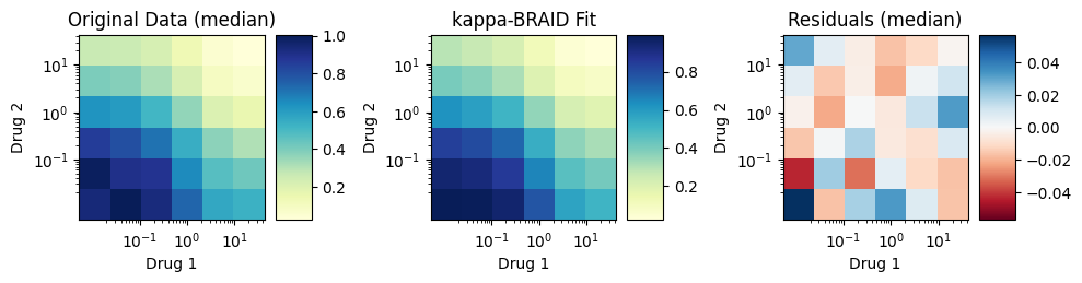
fig = plt.figure(figsize=(10, 5))
plot_heatmap(d1, d2, E, title="Original Data", cmap="YlGnBu", ax=fig.add_subplot(1, 3, 1))
plot_heatmap(unique_d1, unique_d2, model_kappa.E(unique_d1, unique_d2), title="kappa-BRAID Fit", cmap="YlGnBu", ax=fig.add_subplot(1, 3, 2))
plot_heatmap(d1, d2, model_kappa.E(d1, d2) - E, title="Residuals", cmap="RdBu", ax=fig.add_subplot(1, 3, 3), center_on_zero=True)
plt.tight_layout()

../../_images/models_synergy_braid_8_0.png

N-drug Combinations

The BRAID model has not been generalized to an \(N\)-drug case

References

Twarog, N. R., Stewart, E., Hammill, C. V., & Shelat, A. A. (2016). BRAID: A Unifying Paradigm for the Analysis of Combined Drug Action. Scientific reports, 6, 25523. https://doi.org/10.1038/srep25523

[ ]: