HSA

Description

The Highest Single Agent (HSA) model is a dose-dependent synergy model that quantifies synergy based on how much stronger a combination is than the individual constituent single drugs.

\[synergy(d_1, d_2) := \min\left(E_1(d_1), E_2(d_2)\right) - E(d_1, d_2)\]

The values of HSA synergy are interpreted as

Value	Interpretation
\[> 0\]	Synergistic
\[< 0\]	Antagonistic
\[= 0\]	Additive

Assumptions

• None

Defaults

• Single-drug models:

  • Default: synergy.single.log_linear.LogLinear

  • Required: synergy.single.DoseResponse1D or subclass

• Stronger effects are represented by lesser values (i.e., \(E_{\text{strong}} < E_{\text{weak}}\))

  • This is typical in drug studies where the addition of a drug decreases some measured value (e.g., cell counts)

  • This can be overridden by initializing the model as model = HSA(orientation=np.max) in which case the larger E value will be considered as the stronger effect.

2D

Load and plot example dataset

2D synergy models work with 1D arrays of drug 1 dose, drug 2 dose, and effect.

from synergy import datasets
from synergy.utils.plots import plot_heatmap, plot_surface_plotly, set_plotly_interactive

set_plotly_interactive()  # This should only be run in an interactive notebook setting - for other scripts skip this

d1, d2, E = datasets.load_2d_example()

Plot raw dose response data as a heatmap using synergy.utils.plots.plot_heatmap()

plot_heatmap(d1, d2, E, title="Response Data", cmap="YlGnBu")

Plot raw dose response data as a 3D surface with synergy.utils.plots.plot_surface_plotly()

# scatter_points can be used to add a 3d scatter plot over the surface
# plotly's Scatter3D does not appear to work in Jupyter notebooks, but will work if you save the plot to file, e.g., with fname="plot.html"
# scatter_points can be a dict, or a pandas.DataFrame, as long as scatter_points["drug1.conc"], etc return the appropriate arrays.
scatter_points = {
    "drug1.conc": d1,
    "drug2.conc": d2,
    "effect": E
}
plot_surface_plotly(
    d1, d2, E, title="Response Data", cmap="YlGnBu", scatter_points=scatter_points,
    zlabel="Effect"
)  #  fname="plot.html")

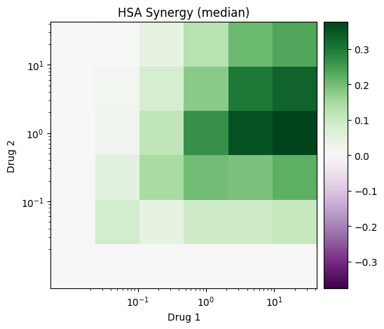
Calculate synergy using the HSA model

from synergy.combination.hsa import HSA

model = HSA()
synergy = model.fit(d1, d2, E)
plot_heatmap(d1, d2, synergy, cmap="PRGn", title="HSA Synergy", center_on_zero=True)
# plot_surface_plotly(d1, d2, synergy, cmap="PRGn", title="HSA Synergy", center_on_zero=True)

N-drug Combinations

The HSA model generalizes to \(N\)-drugs by defining synergy as

\[synergy(\vec{d}) = \min\left(E_i(d_i)\right)\]

Synergy is defined and interpreted identically as in the 2D case.

from synergy.higher.hsa import HSA
from synergy.utils.plots import plotly_isosurfaces
from synergy import datasets

d, E = datasets.load_3d_example()
model = HSA()
synergy = model.fit(d, E)

plotly_isosurfaces(d, E, title="3D Response Data", cmap="YlGnBu")  # or add fname= to save to file
plotly_isosurfaces(d, synergy, title="3D HSA Synergy", cmap="PRGn", center_on_zero=True)

References

Gaddum J. Pharmacology. London: Oxford University Press; 1940.