MuSyC
Description
Multidimensional Synergy of Combinations (MuSyC) is a parametric drug synergy model. Synergy is quantified parametrically as shifts in individual drugs’ potency (alpha), efficacy (beta), or cooperativity (gamma).
It uses a state-transition model to describe drug treatment, in which targets (e.g., cells) are affected or unaffected by each drug. MuSyC fits parameters for the drug-induced effect at each state (efficacy) and dose-induced transitions between states (potency and cooperativity).
synergy.combination.musyc.MuSyC supports two modes
fit_gamma=True(default)Fits all MuSyC synergy parameters, including
gamma
fit_gamma=FalseOnly fits
alphaandbetasynergy parameters, but assumesgamma=1In general
gammais a difficult parameter to fit, unless the combination is much stronger (or weaker) than its constituent drugs. This mode may be prefered if there is insufficient data to fit the full model andgammais not an interesting parameter for the research questions at hand.
The values of MuSyC synergy parameters are interpreted as
Parameter |
Values |
Synergy/Antagonism |
Interpretation |
|---|---|---|---|
alpha12 |
\([0, 1)\) |
Antagonistic Potency |
Drug 1 decreases the effective dose (potency) of drug 2 |
\(> 1\) |
Synergistic Potency |
Drug 1 increases the effective dose (potency) of drug 2 |
|
alpha21 |
\([0, 1)\) |
Antagonistic Potency |
Drug 2 decreases the effective dose (potency) of drug 1 |
\(> 1\) |
Synergistic Potency |
Drug 2 increases the effective dose (potency) of drug 1 |
|
beta |
\(< 0\) |
Antagonistic Efficacy |
The combination is weaker than the stronger of drugs 1 and 2 |
\(> 0\) |
Synergistic Efficacy |
The combination is stronger than the stronger of drugs 1 and 2 |
|
gamma12 |
\([0, 1)\) |
Antagonistic Cooperativity |
Drug 1 decreases the cooperativity (response steepness) of drug 2 |
\(> 1\) |
Synergistic Cooperativity |
Drug 1 increases the cooperativity (response steepness) of drug 2 |
|
gamma21 |
\([0, 1)\) |
Antagonistic Cooperativity |
Drug 2 decreases the cooperativity (response steepness) of drug 1 |
\(> 1\) |
Synergistic Cooperativity |
Drug 2 increases the cooperativity (response steepness) of drug 1 |
Assumptions
Each individual drug follows a Hill equation dose response
Defaults
Single-drug models:
Default:
synergy.single.hill.HillRequired:
synergy.single.hill.Hillor subclass
2D Example
Load example dataset
2D synergy models work with 1D arrays of drug 1 dose, drug 2 dose, and effect.
[1]:
from synergy import datasets
from synergy.utils.plots import plot_heatmap, plot_surface_plotly, set_plotly_interactive

set_plotly_interactive()  # This should only be run in an interactive notebook setting - for other scripts skip this

# datasets.load_2d_example() data was generated with a MuSyC model with
#   beta = 0.25 (synergistic)
#   alpha12 = 2.8 (synergistic)
#   and all other synergistic parameters = 1.0
d1, d2, E = datasets.load_2d_example()
Fit the model to data
Specifying parameter bounds
When reasonable bounds on parameters are known, these bounds can be passed into the model. If you struggle to get good fits, constraining parameters into reasonable ranges can often help.
There are a few ways to do this
Pass bounds for specific parameters:
MuSyC(E0_bounds=(0.9, 1), h1_bounds=(0.5, 2), ....Pass “generic” bounds for whole classes of parameters:
MuSyC(E_bounds=(0, 1), h_bounds=(1e-3, 1e3), alpha_bounds=(1e-3, 1e3), ...).With generic bounds, ALL parameters whose names start with
"E","h","alpha"(etc) will be constrained by the given bounds,
Mix the above:
MuSyC(E_bounds=(0, 1), E0_bounds=(0.9, 1), ...).Specific bounds will always take priority of generic bounds, so this would use
(0.9, 1)forE0, and(0, 1)forE1,E2, andE3.
By default, MuSyC uses bounds of (0, inf) for h, C, alpha, and gamma parameters, and (-inf, inf) for E parameters.
For this synthetic dataset, the data was generated such that E ranges from 0 to 1 (+/- noise, but we can assume all E params should be in that range). So we can pass E_bounds=(0, 1) when we instatiate the MuSyC model.
[2]:
from synergy.combination import MuSyC
import numpy as np

np.random.seed(321)

model = MuSyC(E_bounds=(0, 1))
model.fit(d1, d2, E, bootstrap_iterations=100)  # bootstrap iterations is used to get confidence intervals
model.summarize()  # print a table of synergy parameters, values, confidence intervals, and determination
Parameter  |  Value  |  95% CI          |  Comparison  |  Synergy
=====================================================================
beta       |  0.261  |  (0.175, 0.333)  |  > 0         |  synergistic
alpha12    |  3.54   |  (2.67, 4.93)    |  > 1         |  synergistic
alpha21    |  1.29   |  (0.845, 2.45)   |  ~= 1        |  additive
gamma12    |  0.947  |  (0.762, 1.2)    |  ~= 1        |  additive
gamma21    |  0.722  |  (0.487, 1.2)    |  ~= 1        |  additive
Check model fit quality
All parametric models automatically calculate quality-of-fit scores.
[3]:
print(f"Is fit: {model.is_fit}")  # True if model.fit() was run
print(f"Fit converged: {model.is_converged}")  # True if the model fit successfully converged
print(f"Is fully specified: {model.is_specified}")  # True if all parameters are set (required to call model.E())
print()
print("Fit Quality Stats")
print(f"  Sum of squares residuals: {model.sum_of_squares_residuals}")
print(f"  R^2: {model.r_squared}")
print(f"  AIC: {model.aic}")
print(f"  BIC: {model.bic}")
Is fit: True
Fit converged: True
Is fully specified: True

Fit Quality Stats
  Sum of squares residuals: 0.07890364796738095
  R^2: 0.9915343722513189
  AIC: -750.6549662251795
  BIC: -719.0714707988803
Get all model parameters and confidence intervals
The parameters and confidence intervals are returned by the model as a dict.
Info: For MuSyC, beta is not a parameter that is directly fit, rather it is derived from E0, E1, E2, and E3 which are all fit. As a consequence, model.get_parameters() does not include beta. To get the model’s beta parameter, you must explicitly refer to model.beta. However for convenience, model.get_confidence_intervals() does include beta.
[4]:
print("Parameters:")
parameters = model.get_parameters()
parameters.update({"beta": model.beta})
print(parameters)
print()
print("Confidence Intervals (95%):")
print(model.get_confidence_intervals())  # confidence intervals are stored as lower_bound, upper_bound
print()

# Alternative confidence intervals can also be obtained
print("Confidence Intervals (50%):")
print(model.get_confidence_intervals(confidence_interval=50))
Parameters:
{'E0': 0.999999999596064, 'E1': 0.5120406245501371, 'E2': 0.20668322782869883, 'E3': 2.378729398090393e-13, 'h1': 1.2313572779100372, 'h2': 0.8103212406214214, 'C1': 0.9691712906594294, 'C2': 1.0999704598676796, 'alpha12': 3.544058256487574, 'alpha21': 1.2938532415670458, 'gamma12': 0.9474847282804671, 'gamma21': 0.7220000664387303, 'beta': 0.26053051590981546}

Confidence Intervals (95%):
{'E0': array([0.98141806, 1.        ]), 'E1': array([0.48414389, 0.53881339]), 'E2': array([0.15761893, 0.24764064]), 'E3': array([2.11043724e-22, 3.06019107e-02]), 'h1': array([1.02532838, 1.51207123]), 'h2': array([0.7138909 , 0.91495537]), 'C1': array([0.84735083, 1.15779538]), 'C2': array([0.93764325, 1.4144282 ]), 'alpha12': array([2.67065667, 4.93170657]), 'alpha21': array([0.84522653, 2.45207853]), 'gamma12': array([0.76236592, 1.20186368]), 'gamma21': array([0.48697516, 1.20048448]), 'beta': array([0.17520408, 0.33292308])}

Confidence Intervals (50%):
{'E0': array([0.99274493, 1.        ]), 'E1': array([0.49921397, 0.51980405]), 'E2': array([0.19040288, 0.2255272 ]), 'E3': array([4.50473383e-15, 9.90354476e-03]), 'h1': array([1.15343766, 1.32978216]), 'h2': array([0.78391239, 0.86193039]), 'C1': array([0.93368586, 1.05953768]), 'C2': array([1.03899173, 1.21267708]), 'alpha12': array([3.1930444 , 4.22264247]), 'alpha21': array([1.16599156, 1.70885191]), 'gamma12': array([0.89903748, 1.0185653 ]), 'gamma21': array([0.64715026, 0.90553719]), 'beta': array([0.22975415, 0.28117074])}
Plot the model fit
[5]:
from synergy.utils.dose_utils import make_dose_grid

# Get a smooth looking dose response surface from dmin=0.025 to dmax=20
dmin, dmax = 0.025, 20
n_points = 20  # 20 points x 20 points
d1_smooth, d2_smooth = make_dose_grid(dmin, dmax, dmin, dmax, n_points, n_points)
E_smooth = model.E(d1_smooth, d2_smooth)

scatter_points = {
    "drug1.conc": d1,
    "drug2.conc": d2,
    "effect": E
}

plot_surface_plotly(d1_smooth, d2_smooth, E_smooth, cmap="YlGnBu", title="MuSyC Fit", scatter_points=scatter_points)
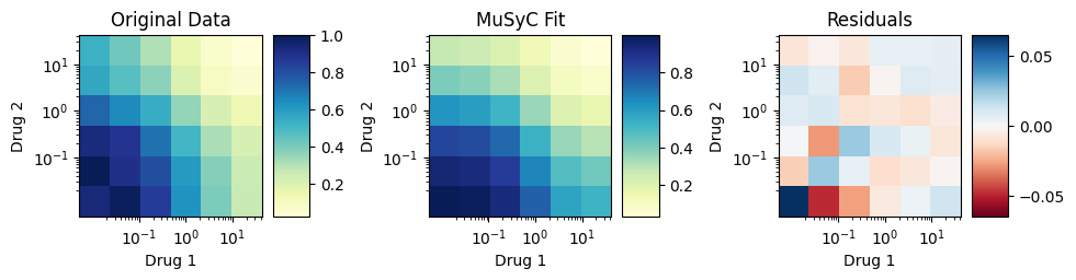
[6]:
from matplotlib import pyplot as plt
import numpy as np

from synergy.utils.dose_utils import aggregate_replicates

# plot_heatmap will automatically aggregate replicates for real data, but we don't need it to do that for the MuSyC fit
d, _ = aggregate_replicates(np.vstack([d1, d2]).transpose(), E)
unique_d1 = d[:, 0]
unique_d2 = d[:, 1]

fig = plt.figure(figsize=(10, 5))
plot_heatmap(d1, d2, E, title="Original Data", cmap="YlGnBu", ax=fig.add_subplot(1, 3, 1))
plot_heatmap(unique_d1, unique_d2, model.E(unique_d1, unique_d2), title="MuSyC Fit", cmap="YlGnBu", ax=fig.add_subplot(1, 3, 2))
plot_heatmap(d1, d2, model.E(d1, d2) - E, title="Residuals", cmap="RdBu", ax=fig.add_subplot(1, 3, 3), center_on_zero=True)
plt.tight_layout()
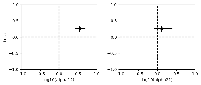
Plot drug synergy diagram
[7]:
from matplotlib import pyplot as plt
import numpy as np

confidence_intervals = model.get_confidence_intervals()  # defaults to 95% confidence interval
beta = model.beta
beta_ci = confidence_intervals["beta"]
alpha12 = np.log10(model.alpha12)  # It is recommended to visualize log(alpha) so antagonism < 0, synergism > 0
alpha12_ci = np.log10(confidence_intervals["alpha12"])
alpha21 = np.log10(model.alpha21)
alpha21_ci = np.log10(confidence_intervals["alpha21"])

fig = plt.figure(figsize=(7,3))

ax = fig.add_subplot(1, 2, 1)
ax.scatter([alpha12], [beta], c="k")
ax.plot(alpha12_ci, [beta, beta], "k-")
ax.plot([alpha12, alpha12], beta_ci, "k-")
ax.set_xlabel("log10(alpha12)")
ax.set_ylabel("beta")
ax.axhline(y=0, c="k", ls="--")
ax.axvline(x=0, c="k", ls="--")
ax.set_xlim(-1, 1)
ax.set_ylim(-1, 1)

ax = fig.add_subplot(1, 2, 2)
ax.scatter([alpha21], [beta], c="k")
ax.plot(alpha21_ci, [beta, beta], "k-")
ax.plot([alpha21, alpha21], beta_ci, "k-")
ax.set_xlabel("log10(alpha21)")
ax.axhline(y=0, c="k", ls="--")
ax.axvline(x=0, c="k", ls="--")
ax.set_xlim(-1, 1)
ax.set_ylim(-1, 1)

plt.tight_layout()
plt.show()
N-drug Example (N > 2)
Description
The MuSyC model is generalized to \(N\)-drugs, but adds many more parameters to be fit.
Parameter |
Number of parameters |
|---|---|
E |
\(2^N\) |
h |
\(N\) |
C |
\(N\) |
alpha |
\(N \cdot \left(2^{N-1} - 1\right)\) |
beta* |
\(2^N - N - 1\) |
gamma** |
\(N \cdot \left(2^{N-1} - 1\right)\) |
*beta does not need to be fit on its own - rather it is derived from the \(E\) parameters.
**gamma is only fit if the model is instantiated with
MuSyC(fit_gamma=True), which isFalseby defualt.
The parameter’s names follow the following conventions
Single drug parameters
E_ih_iC_i
Combination parameters
E_i,j,...Examples
E_1,2: E at saturating concentrations of drugs 1 and 2E_2,3,4: E at saturating concentrations of drugs 2, 3, and 4
alpha_i,j,..._kExamples
alpha_1,2: the impact of drug 1 on drug 2’s potencyalpha_2,3_1: the impact of drugs 2 and 3 together on drug 1’s potency
beta_i,j,...Examples
beta_1,2: the strength of the combination of drugs 1 and 2 relative to the stronger of drugs 1 or 2 alonebeta_1,2,3: the strength of the combination of drugs 1, 2, and 3 relative to the strongest combination of drugs 1 and 2, drugs 2 and 3, or drugs 1 and 3
gamma_i,j,..._kExamples
gamma_1,2: the impact of drug 1 on drug 2’s cooperativitygamma_2,3_1: the impact of drugs 2 and 3 together on drug 1’s cooperativity
The values of synergy parameters are interpreted identically as in the 2D case.
Load example dataset
datasets.load_3d_example() data was generated with a MuSyC model with
beta_1,2 = 0(additive)beta_1,3 = -0.083(weakly antagonistic)beta_2,3 = 0.5(synergistic)beta_1,2,3 = 0.25(synergistic)alpha_3_2 = 0.5(antagonistic)alpha_2,3_1 = 3.0(synergistic)all other synergistic parameters = 1.0
[8]:
from synergy.higher import MuSyC as MuSyCND
from synergy import datasets

d, E = datasets.load_3d_example()
Fit the model to data
[9]:
np.random.seed(1111)

model = MuSyCND(num_drugs=3)
model.fit(d, E, bootstrap_iterations=100, use_jacobian=False)
model.summarize()
Parameter    |  Value   |  95% CI             |  Comparison  |  Synergy
============================================================================
beta_1,2     |  0.0756  |  (-0.0491, 0.207)   |  ~= 0        |  additive
beta_1,3     |  -0.129  |  (-0.198, -0.0793)  |  < 0         |  antagonistic
beta_2,3     |  0.327   |  (0.253, 0.408)     |  > 0         |  synergistic
beta_1,2,3   |  0.239   |  (0.163, 0.323)     |  > 0         |  synergistic
alpha_1_3    |  1.35    |  (0.928, 1.89)      |  ~= 1        |  additive
alpha_1_2    |  0.38    |  (0.132, 0.979)     |  < 1         |  antagonistic
alpha_2_3    |  1       |  (0.681, 1.37)      |  ~= 1        |  additive
alpha_2_1    |  0.821   |  (0.106, 1.96)      |  ~= 1        |  additive
alpha_1,2_3  |  0.869   |  (0.511, 1.23)      |  ~= 1        |  additive
alpha_3_2    |  0.594   |  (0.212, 1.26)      |  ~= 1        |  additive
alpha_3_1    |  0.427   |  (0.0462, 1.82)     |  ~= 1        |  additive
alpha_1,3_2  |  1.57    |  (0.871, 2.91)      |  ~= 1        |  additive
alpha_2,3_1  |  3.51    |  (2.28, 4.67)       |  > 1         |  synergistic
[10]:
from synergy.utils.plots import plotly_isosurfaces
from synergy.utils.dose_utils import make_dose_grid_multi


# Get a smooth looking dose response surface from dmin=0.025 to dmax=20
dmin, dmax = [0.025] * 3, [20] * 3
n_points = [20] * 3  # 20 points x 20 points x 20 points
d_smooth = make_dose_grid_multi(dmin, dmax, n_points)

plotly_isosurfaces(d, E, title="3D Original Data", cmap="YlGnBu")  # or add fname= to save to file
plotly_isosurfaces(d_smooth, model.E(d_smooth), title="3D MuSyC Fit", cmap="YlGnBu")
Get all model parameters and confidence intervals
[11]:
print("Parameters:")
parameters = model.get_parameters()
parameters.update(model.beta)
print(parameters)
print()

# confidence intervals are stored as lower_bound, upper_bound
print("Confidence Intervals (95%):")
print(model.get_confidence_intervals())
print()

# Alternative confidence intervals can also be obtained
print("Confidence Intervals (50%):")
print(model.get_confidence_intervals(confidence_interval=50))
Parameters:
{'E_0': 0.990549246251572, 'E_1': 0.6891048485235974, 'E_2': 0.4986418092080175, 'E_1,2': 0.46143478126233095, 'E_3': 0.3968071882049947, 'E_1,3': 0.47355693866849735, 'E_2,3': 0.2027211237498031, 'E_1,2,3': 0.014642659372348934, 'h_1': 2.232676239536823, 'h_2': 0.5046476751827258, 'h_3': 1.0032971586214017, 'C_1': 1.0653005143136753, 'C_2': 1.0131690307204928, 'C_3': 1.0759057657832176, 'alpha_1_3': 1.350909495239142, 'alpha_1_2': 0.38043457166095934, 'alpha_2_3': 1.0040692732198784, 'alpha_2_1': 0.8210732229373959, 'alpha_1,2_3': 0.8687207695269863, 'alpha_3_2': 0.5935400565195599, 'alpha_3_1': 0.4268817515037964, 'alpha_1,3_2': 1.5722814235757145, 'alpha_2,3_1': 3.506454442471727, 'beta_1,2': 0.07563827082856676, 'beta_1,3': -0.12926446665410696, 'beta_2,3': 0.3268861651703409, 'beta_1,2,3': 0.2387303258231073}

Confidence Intervals (95%):
{'E_0': array([0.97555356, 0.99983074]), 'E_1': array([0.67451495, 0.70492931]), 'E_2': array([0.43916706, 0.53348474]), 'E_1,2': array([0.40347411, 0.50130637]), 'E_3': array([0.37654039, 0.41453507]), 'E_1,3': array([0.45074151, 0.51720521]), 'E_2,3': array([0.16038068, 0.23129103]), 'E_1,2,3': array([-0.05620487,  0.05171532]), 'h_1': array([1.8577313 , 3.57566083]), 'h_2': array([0.44762949, 0.55432417]), 'h_3': array([0.94491257, 1.05864911]), 'C_1': array([0.95555549, 1.22296468]), 'C_2': array([0.69163516, 1.8999261 ]), 'C_3': array([0.96726657, 1.26285426]), 'alpha_1_3': array([0.92761865, 1.88919736]), 'alpha_1_2': array([0.13177768, 0.97886056]), 'alpha_2_3': array([0.68142855, 1.36515066]), 'alpha_2_1': array([0.10642622, 1.96488095]), 'alpha_1,2_3': array([0.5113879 , 1.22781685]), 'alpha_3_2': array([0.21155807, 1.25958945]), 'alpha_3_1': array([0.04617349, 1.81925841]), 'alpha_1,3_2': array([0.87054021, 2.91334387]), 'alpha_2,3_1': array([2.28288093, 4.67425577]), 'beta_1,2': array([-0.04911908,  0.20727998]), 'beta_1,3': array([-0.1982522, -0.0793158]), 'beta_2,3': array([0.2530003 , 0.40817199]), 'beta_1,2,3': array([0.1627866 , 0.32316992])}

Confidence Intervals (50%):
{'E_0': array([0.98386906, 0.99442961]), 'E_1': array([0.68351825, 0.69587124]), 'E_2': array([0.48361346, 0.50999664]), 'E_1,2': array([0.43891796, 0.47761815]), 'E_3': array([0.38790253, 0.40257734]), 'E_1,3': array([0.46582462, 0.48321314]), 'E_2,3': array([0.18466224, 0.20866691]), 'E_1,2,3': array([-0.00485489,  0.03016489]), 'h_1': array([2.07663193, 2.67816945]), 'h_2': array([0.48439544, 0.52511318]), 'h_3': array([0.97503591, 1.03006629]), 'C_1': array([1.02161733, 1.11903745]), 'C_2': array([0.884118  , 1.19332234]), 'C_3': array([1.04187735, 1.13044351]), 'alpha_1_3': array([1.20578897, 1.58845626]), 'alpha_1_2': array([0.23943365, 0.59202679]), 'alpha_2_3': array([0.86719817, 1.10828068]), 'alpha_2_1': array([0.57863183, 1.03505897]), 'alpha_1,2_3': array([0.74519695, 1.01568769]), 'alpha_3_2': array([0.40268124, 0.81154624]), 'alpha_3_1': array([0.23233913, 0.73923069]), 'alpha_1,3_2': array([1.34781828, 1.98198008]), 'alpha_2,3_1': array([3.13202427, 4.01198709]), 'beta_1,2': array([0.03616058, 0.11878208]), 'beta_1,3': array([-0.15196528, -0.11974255]), 'beta_2,3': array([0.30704343, 0.35598056]), 'beta_1,2,3': array([0.2130466 , 0.25840745])}
Since computing confidence intervals can be expensive, an alternative is to use a predefined tolerance passed to summarize(tol=tol). tol for alpha and gamma applies to those parameters on a log-scale, rather than linear scale.
[12]:
np.random.seed(123)
model_no_ci = MuSyCND(num_drugs=3)
model_no_ci.fit(d, E, use_jacobian=False)
model_no_ci.summarize(tol=0.3)
Parameter    |  Value   |  Comparison  |  Synergy
======================================================
beta_1,2     |  0.0756  |  ~= 0        |  additive
beta_1,3     |  -0.129  |  ~= 0        |  additive
beta_2,3     |  0.327   |  > 0         |  synergistic
beta_1,2,3   |  0.239   |  ~= 0        |  additive
alpha_1_3    |  1.35    |  > 1         |  synergistic
alpha_1_2    |  0.38    |  < 1         |  antagonistic
alpha_2_3    |  1       |  ~= 1        |  additive
alpha_2_1    |  0.821   |  ~= 1        |  additive
alpha_1,2_3  |  0.869   |  ~= 1        |  additive
alpha_3_2    |  0.594   |  < 1         |  antagonistic
alpha_3_1    |  0.427   |  < 1         |  antagonistic
alpha_1,3_2  |  1.57    |  > 1         |  synergistic
alpha_2,3_1  |  3.51    |  > 1         |  synergistic
References
Meyer, Christian T., et al. “Quantifying drug combination synergy along potency and efficacy axes.” Cell systems 8.2 (2019): 97-108.
Wooten, David J., et al. “MuSyC is a consensus framework that unifies multi-drug synergy metrics for combinatorial drug discovery.” Nature communications 12.1 (2021): 4607.
[ ]: