Hill

Description

The Hill equation is a parametric dose-response model derived from chemical kinetics. It has a sigmoidal shape when plotting against log-scaled doses. It contains the following parameters

Parameter	Description
E0	Effect when \(d=0\)
Emax	Asymptotic effect as \(d \rightarrow \infty\)
C	Dose such that \(E(d=C) = \frac{E_0 + E_\text{max}}{2}\)
h	“Hill coefficient” related to the slope near \(d=C\)

There are two public subclasses of synergy.single.hill.Hill

• Hill_2P

  • This model does not fit E0 or Emax, but rather expects them to be supplied when the model is instantiated.

• Hill_CI

  • This model is a further subclass of Hill_2P with E0=1.0 and Emax=0.0. Additionally, it fits the dose-response curve using the linearization method of the median effect equation, rather than via scipy.optimize.curve_fit().

Assumptions

• The data should follow a sigmoidal shape

If the assumptions are not met, you may consider using a different single-drug model, such as LogLinear.

Hill Example

Fit the model to data

Dose response models work with 1D arrays of E and drug dose.

Specifying parameter bounds

When reasonable bounds on parameters are known, these bounds can be passed into the model. If you struggle to get good fits, constraining parameters into reasonable ranges can often help.

There are a few ways to do this

• Pass bounds for specific parameters: Hill(E0_bounds=(0.9, 1), h_bounds=(0.5, 2), ....

• Pass “generic” bounds for E: Hill(E_bounds=(0, 1), h_bounds=(1e-3, 1e3).

  • With generic bounds, both E0 and Emax will be constrained by the given bounds,

• Mix the above: Hill(E_bounds=(0, 1), E0_bounds=(0.9, 1), ...).

  • Specific bounds will always take priority of generic bounds, so this would use (0.9, 1) for E0, and (0, 1) for Emax.

By default, Hill uses bounds of (0, inf) for h and C, and (-inf, inf) for E parameters.

For this synthetic dataset, the data was generated such that E ranges from 0 to 1 (+/- noise, but we can assume all E params should be in that range). So we can pass E_bounds=(0, 1) when we instatiate the model.

import numpy as np

from synergy import datasets
from synergy.single import Hill

np.random.seed(1234)  # deterministic confidence intervals

d, E = datasets.load_hill_example()
model = Hill(E_bounds=(-0.1, 1.1))
model.fit(d, E, bootstrap_iterations=100)  # bootstrap_iterations is used to estimate confidence intervals

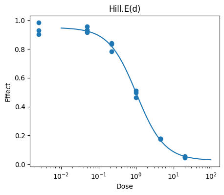
Plot the model fit

from matplotlib import pyplot as plt

from synergy.utils import remove_zeros

fig = plt.figure(figsize=(5, 4))
ax = fig.add_subplot(1, 1, 1)
ax.scatter(remove_zeros(d, num_dilutions=2), E)

# This is used as the x-axis values for model.E(d), to give a smooth curve
d_smooth = np.logspace(-2, 2)
ax.plot(d_smooth, model.E(d_smooth))
ax.set_xscale("log")
ax.set_xlabel("Dose")
ax.set_ylabel("Effect")
ax.set_title("Hill.E(d)")
plt.show()

Check model fit quality

All parametric models automatically calculate quality-of-fit scores.

print(f"Is fit: {model.is_fit}")  # True if model.fit() was run
print(f"Fit converged: {model.is_converged}")  # True if the model fit successfully converged
print(f"Is fully specified: {model.is_specified}")  # True if all parameters are set (required to call model.E())
print()
print("Fit Quality Stats")
print(f"  Sum of squares residuals: {model.sum_of_squares_residuals}")
print(f"  R^2: {model.r_squared}")
print(f"  AIC: {model.aic}")
print(f"  BIC: {model.bic}")

Is fit: True
Fit converged: True
Is fully specified: True

Fit Quality Stats
  Sum of squares residuals: 0.008834185033397293
  R^2: 0.996153655058854
  AIC: -124.07404413296418
  BIC: -122.69910842040643

Get all model parameters and confidence intervals

print("Parameters")
print(model.get_parameters())
print()

print("Confidence Interval (95%)")
print(model.get_confidence_intervals())
print()

print("Confidence Interval (50%)")
print(model.get_confidence_intervals(confidence_interval=50))
print()

Parameters
{'E0': 0.9486656324539504, 'Emax': 0.02687061853180388, 'h': 1.1734807393913014, 'C': 1.034970209440454}

Confidence Interval (95%)
{'E0': array([0.92956039, 0.97436566]), 'Emax': array([-0.00384545,  0.06494899]), 'h': array([1.03013288, 1.35836766]), 'C': array([0.92052359, 1.16038919])}

Confidence Interval (50%)
{'E0': array([0.94089162, 0.95468789]), 'Emax': array([0.0181467 , 0.04309284]), 'h': array([1.12620809, 1.2573561 ]), 'C': array([0.98274748, 1.07777016])}

Hill_2P Example

from synergy.single import Hill_2P

np.random.seed(1234)  # deterministic confidence intervals

d, E = datasets.load_hill_example()
model_2p = Hill_2P(E0=1.0, Emax=0.0)
model_2p.fit(d, E, bootstrap_iterations=100)

Plot and analyze Hill_2P fit

fig = plt.figure(figsize=(5, 4))
ax = fig.add_subplot(1, 1, 1)
ax.scatter(remove_zeros(d, num_dilutions=2), E)

# This is used as the x-axis values for model.E(d), to give a smooth curve
d_smooth = np.logspace(-2, 2)
ax.plot(d_smooth, model_2p.E(d_smooth))
ax.set_xscale("log")
ax.set_xlabel("Dose")
ax.set_ylabel("Effect")
ax.set_title("Hill_2P.E(d)")
plt.show()

print("\n===\n")
print("Model Fit Scores")

print(f"Is fit: {model_2p.is_fit}")  # True if model.fit() was run
print(f"Fit converged: {model_2p.is_converged}")  # True if the model fit successfully converged
print(f"Is fully specified: {model_2p.is_specified}")  # True if all parameters are set (required to call model.E())
print()
print("Fit Quality Stats")
print(f"  Sum of squares residuals: {model_2p.sum_of_squares_residuals}")
print(f"  R^2: {model_2p.r_squared}")
print(f"  AIC: {model_2p.aic}")
print(f"  BIC: {model_2p.bic}")

print("\n===\n")
print("Model Parameters")

print("Parameters")
print(model_2p.get_parameters())
print()

print("Confidence Interval (95%)")
print(model_2p.get_confidence_intervals())
print()

print("Confidence Interval (50%)")
print(model_2p.get_confidence_intervals(confidence_interval=50))
print()

===

Model Fit Scores
Is fit: True
Fit converged: True
Is fully specified: True

Fit Quality Stats
  Sum of squares residuals: 0.02024364996923748
  R^2: 0.9911860505122833
  AIC: -115.42514573683924
  BIC: -113.55403046315075

===

Model Parameters
Parameters
{'h': 0.9954835060681304, 'C': 0.9678777475974989}

Confidence Interval (95%)
{'h': array([0.90821956, 1.11325105]), 'C': array([0.87306605, 1.0633984 ])}

Confidence Interval (50%)
{'h': array([0.95776381, 1.04535511]), 'C': array([0.93218408, 1.01349353])}

Hill_CI Example

from synergy.single import Hill_CI

d, E = datasets.load_hill_example()
model_ci = Hill_CI()  # parameter bounds are not yet supported for Hill_CI
model_ci.fit(d, E)  # confidence intervals are not yet supported for Hill_CI

Plot and analyze Hill_CI fit

fig = plt.figure(figsize=(5, 4))
ax = fig.add_subplot(1, 1, 1)
ax.scatter(remove_zeros(d, num_dilutions=2), E)

# This is used as the x-axis values for model.E(d), to give a smooth curve
d_smooth = np.logspace(-2, 2)
ax.plot(d_smooth, model_ci.E(d_smooth))
ax.set_xscale("log")
ax.set_xlabel("Dose")
ax.set_ylabel("Effect")
ax.set_title("Hill_CI.E(d)")
plt.show()

print("\n===\n")
print("Model Fit Scores")

print(f"Is fit: {model_ci.is_fit}")  # True if model.fit() was run
print(f"Fit converged: {model_ci.is_converged}")  # True if the model fit successfully converged
print(f"Is fully specified: {model_ci.is_specified}")  # True if all parameters are set (required to call model.E())
print()
print("Fit Quality Stats")
print(f"  Sum of squares residuals: {model_ci.sum_of_squares_residuals}")
print(f"  R^2: {model_ci.r_squared}")
print(f"  AIC: {model_ci.aic}")
print(f"  BIC: {model_ci.bic}")

print("\n===\n")
print("Model Parameters")

print("Parameters")
print(model_ci.get_parameters())
print()

===

Model Fit Scores
Is fit: True
Fit converged: True
Is fully specified: True

Fit Quality Stats
  Sum of squares residuals: 0.02105340328571227
  R^2: 0.9908334893466948
  AIC: -114.71916664367039
  BIC: -112.8480513699819

===

Model Parameters
Parameters
{'h': 0.9627465059253871, 'C': 0.9361750189247218}

References

Chou, Ting‐Chao, and Paul TaLaLay. “Generalized equations for the analysis of inhibitions of Michaelis‐Menten and higher‐order kinetic systems with two or more mutually exclusive and nonexclusive inhibitors.” European journal of biochemistry 115.1 (1981): 207-216.